From: https://github.com/ksatola
Version: 0.1.0
Model - PM2.5 - AutoRegressive Moving Average (ARMA)
Contents
- AutoRegressive Moving Average (ARMA) modelling
- Hourly forecast
- Daily forecast
%load_ext autoreload
%autoreload 2
import sys
sys.path.insert(0, '../src')
import warnings
warnings.filterwarnings('ignore')

from statsmodels.tools.sm_exceptions import ConvergenceWarning, ValueWarning
warnings.simplefilter('ignore', ConvergenceWarning)
warnings.simplefilter('ignore', ValueWarning)
import pandas as pd
import numpy as np

from statsmodels.tsa.statespace.sarimax import SARIMAX

import matplotlib.pyplot as plt
%matplotlib inline
from model import (
    get_pm25_data_for_modelling,
    get_best_arima_params_for_time_series,
    split_df_for_ts_modelling_offset,
    predict_ts,
    fit_model
)

from measure import (
    get_rmse,
    walk_forward_ts_model_validation2,
    get_mean_folds_rmse_for_n_prediction_points,
    prepare_data_for_visualization
)

from plot import (
    visualize_results,
    plot_ts_corr
)

from utils import (
    get_datetime_identifier
)

from logger import logger
model_name = 'ARMA'
Autoregressive Moving Average (ARMA) modelling
An ARMA model, or Autoregressive Moving Average model, is used to describe weakly stationary stochastic time series in terms of two polynomials. The first of these polynomials is for autoregression (AR), the second for the moving average (MA):
AR(p) uses previous values of the dependent variable to make predictions.
MA(q) uses the series mean and previous errors to make predictions.
Often this model is referred to as the ARMA(p,q) model; where:
p is the order of the autoregressive polynomial,
q is the order of the moving average polynomial.
The equation is given by:
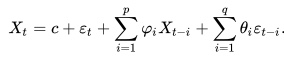
Where:
φ = the autoregressive model’s parameters,
θ = the moving average model’s parameters.
c = a constant,
ε = error terms (white noise).
The Time Series ARMA Forecasting Process
- Perform simple time series EDA
- Missing observations
- Data centricity and spread
- Outliers, trend and frequency changes -> stationarity, detrending?
- Data distribution fit into Gaussian distribution -> power transforms?
- Perform TS Decomposition, take residuals for the modeling
- Test stationarity of residuals
- Check if residuals is white noise
- Split the residuals dataset into train, test sets
dfh = get_pm25_data_for_modelling('ts', 'h')
dfh.head()
df = dfh.copy()
# Define first past/future cutoff point in time offset (1 year of data)
cut_off_offset = 365*24 # for hourly data
#cut_off_offset = 365 # for daily data

# Predict for X points
n_pred_points = 24 # for hourly data
#n_pred_points = 7 # for daily data

# https://pandas.pydata.org/pandas-docs/stable/user_guide/timeseries.html#offset-aliases
period = 'H' # for hourly data
#period = 'D' # for daily data
Train test split
# Create train / test datasets (with the offset of cut_off_offset datapoints from the end)
# period=None because we need index to be DatetimeIndex not PeriodIndex for SARIMAX
df_train, df_test = split_df_for_ts_modelling_offset(data=df, cut_off_offset=cut_off_offset, period=None)
Modelling (train, predict/validate)
In statistical time series models, fitting the model means estimating its paraneters. In case of AR model, the only parameter to estimate is number of autocorrelated lags.
plot_ts_corr(df_train['pm25'])

%%time
# Find best parameters (grid-search)
best_results = get_best_arima_params_for_time_series(data=df_train,
                                                     seasonal=False,
                                                     max_param_range_p=5,
                                                     max_param_range_d=2,
                                                     max_param_range_q=5)
SARIMAX(0, 0, 0) - AIC:950035.119919657
SARIMAX(0, 0, 1) - AIC:843344.0396508672
SARIMAX(0, 0, 2) - AIC:772685.05307077
SARIMAX(0, 0, 3) - AIC:726435.4649042541
SARIMAX(0, 0, 4) - AIC:699267.5669061132
SARIMAX(0, 0, 5) - AIC:679220.6801305263
SARIMAX(0, 1, 0) - AIC:637526.5016885484
SARIMAX(0, 1, 1) - AIC:629960.3879021691
SARIMAX(0, 1, 2) - AIC:628846.653452479
SARIMAX(0, 1, 3) - AIC:628480.5779072419
SARIMAX(0, 1, 4) - AIC:628474.1076286844
SARIMAX(0, 1, 5) - AIC:628470.5808444964
SARIMAX(1, 0, 2) - AIC:627752.667749163
SARIMAX(1, 0, 3) - AIC:627233.671710295
SARIMAX(1, 0, 4) - AIC:627176.4310598889
SARIMAX(1, 0, 5) - AIC:627165.0028807595
SARIMAX(1, 1, 3) - AIC:626081.1199039271
SARIMAX(1, 1, 5) - AIC:625019.2327505194
SARIMAX(2, 1, 2) - AIC:624910.203481772
SARIMAX(2, 1, 3) - AIC:624873.0049011122
SARIMAX(2, 1, 4) - AIC:624854.8941542685
SARIMAX(3, 0, 3) - AIC:624793.04465309
SARIMAX(5, 0, 2) - AIC:624767.846410448
SARIMAX(5, 0, 3) - AIC:624676.504781964
Best model is ARIMA(5, 0, 3) with AIC of 624676.504781964
CPU times: user 2h 35min 14s, sys: 15min 17s, total: 2h 50min 32s
Wall time: 49min 34s
%%time
# Train the model -> find best parameters
p = 5 # (AR)
d = 0 # differencing
q = 3 # (MA)
model = SARIMAX(endog=df_train, order=(p, d, q))
model_fitted = model.fit()
model_fitted
# Estimated parameters
print(model_fitted.summary())
# True parameters
print(f'The coefficients of the model are:\n {model_fitted.params}')
print(f'The residual errors during training of the model are:\n {model_fitted.resid}')
# Evaluate model quality
import statsmodels.api as sm
res = model_fitted.resid
fig,ax = plt.subplots(2,1,figsize=(15,8))
fig = sm.graphics.tsa.plot_acf(res, lags=50, ax=ax[0])
fig = sm.graphics.tsa.plot_pacf(res, lags=50, ax=ax[1])
plt.show();

# Evaluate model quality
model_fitted.plot_diagnostics(figsize=(20, 10))
plt.show();

ARMA model alone fits not vary bad for hourly data but it does not capture the multilayer seasonality (yearly, weekly, daily) in data. There is still way for improvement (if possible).
%%time
# Validate result on test
# Creates 365*24*24 models for hourly data, or 365*7 models for hourly data

fold_results = walk_forward_ts_model_validation2(data=df,
                                                 col_name='pm25',
                                                 model_type='ARMA',
                                                 p=p,
                                                 d=d,
                                                 q=q,
                                                 cut_off_offset=cut_off_offset,
                                                 n_pred_points=n_pred_points,
                                                 n_folds=-1,
                                                 period=period)
print(len(fold_results))
print(fold_results[0])
Serialize output data
from joblib import dump, load

timestamp = get_datetime_identifier("%Y-%m-%d_%H-%M-%S")

path = f'results/pm25_ts_{model_name}_results_h_{timestamp}.joblib'

#dump(fold_results, path)
fold_results = load(path)
print(len(fold_results))
print(fold_results[0])
Calculate and visualize results
%%time
# Returns a list of mean folds RMSE for n_pred_points (starting at 1 point forecast)
res = get_mean_folds_rmse_for_n_prediction_points(fold_results=fold_results, n_pred_points=n_pred_points)
res
print(res)
# Show forecasts for n-th point in the future
show_n_points_of_forecasts = [1, 12, 24] # for hourly data
#show_n_points_of_forecasts = [1, 3, 7] # for daily data

# Used to zoom the plots (date ranges shown in the plots)
# for hourly data
start_end_dates = [('2018-01-01', '2019-01-01'), ('2018-02-01', '2018-03-01'), ('2018-06-01', '2018-07-01')]
# for daily data
#start_end_dates = [('2018-01-01', '2019-01-01'), ('2018-02-01', '2018-04-01'), ('2018-06-01', '2018-08-01')]

# Type of plot
# 0 -> plot_observed_vs_predicted
# 1 -> plot_observed_vs_predicted_with_error
plot_types = [0, 1, 1]

# File names for plots (format png will be used, do not add .png extension)
base_file_path = f'images/pm25_obs_vs_pred_365_h_ts_{model_name}' # for hourly data
#base_file_path = f'images/pm25_obs_vs_pred_365_d_ts_{model_name}' # for daily data
fold_results[0].index
# We need to convert to datetime index for plotting
# https://stackoverflow.com/questions/29394730/converting-periodindex-to-datetimeindex
for i in range(0, len(fold_results)):
    if not isinstance(fold_results[i].index, pd.DatetimeIndex):
        fold_results[i].index = fold_results[i].index.to_timestamp()
fold_results[0].index
visualize_results(show_n_points_of_forecasts=show_n_points_of_forecasts,
                   start_end_dates=start_end_dates,
                   plot_types=plot_types,
                   base_file_path=base_file_path,
                   fold_results=fold_results,
                   n_pred_points=n_pred_points,
                   cut_off_offset=cut_off_offset,
                   model_name=model_name,
                timestamp=timestamp)
dfd = get_pm25_data_for_modelling('ts', 'd')
dfd.head()
df = dfd.copy()
# Define first past/future cutoff point in time offset (1 year of data)
#cut_off_offset = 365*24 # for hourly data
cut_off_offset = 365 # for daily data

# Predict for X points
#n_pred_points = 24 # for hourly data
n_pred_points = 7 # for daily data

# https://pandas.pydata.org/pandas-docs/stable/user_guide/timeseries.html#offset-aliases
#period = 'H' # for hourly data
period = 'D' # for daily data
Train test split
# Create train / test datasets (with the offset of cut_off_offset datapoints from the end)
# period=None because we need index to be DatetimeIndex not PeriodIndex for SARIMAX
df_train, df_test = split_df_for_ts_modelling_offset(data=df, cut_off_offset=cut_off_offset, period=None)
plot_ts_corr(df_train['pm25'])

%%time
# Find best parameters (grid-search)
best_results = get_best_arima_params_for_time_series(data=df_train,
                                                     seasonal=False,
                                                     max_param_range_p=5,
                                                     max_param_range_d=0,
                                                     max_param_range_q=5)
SARIMAX(0, 0, 0) - AIC:38983.00813026588
SARIMAX(0, 0, 1) - AIC:36059.690659735024
SARIMAX(0, 0, 2) - AIC:34918.45008233713
SARIMAX(0, 0, 3) - AIC:34409.81571434598
SARIMAX(0, 0, 4) - AIC:34096.090358520945
SARIMAX(0, 0, 5) - AIC:33892.384328226864
SARIMAX(1, 0, 0) - AIC:33340.065325479634
SARIMAX(1, 0, 1) - AIC:33319.44543874674
SARIMAX(1, 0, 2) - AIC:32936.30774547422
SARIMAX(1, 0, 3) - AIC:32824.261541303546
SARIMAX(1, 0, 4) - AIC:32809.033323439486
SARIMAX(1, 0, 5) - AIC:32805.637460981045
SARIMAX(2, 0, 2) - AIC:32803.919187166546
SARIMAX(4, 0, 4) - AIC:32803.501675630905
SARIMAX(5, 0, 4) - AIC:32802.877819381196
Best model is ARIMA(5, 0, 4) with AIC of 32802.877819381196
CPU times: user 2min 4s, sys: 19.3 s, total: 2min 23s
Wall time: 36 s
%%time
# Train the model -> find best parameters
p = 5 # (AR)
d = 0 # differencing
q = 4 # (MA)
model = SARIMAX(endog=df_train['pm25'], order=(p, d, q))
model_fitted = model.fit()
model_fitted
# Estimated parameters
print(model_fitted.summary())
# True parameters
print(f'The coefficients of the model are:\n {model_fitted.params}')
print(f'The residual errors during training of the model are:\n {model_fitted.resid}')
# Evaluate model quality
import statsmodels.api as sm
res = model_fitted.resid
fig,ax = plt.subplots(2,1,figsize=(15,8))
fig = sm.graphics.tsa.plot_acf(res, lags=50, ax=ax[0])
fig = sm.graphics.tsa.plot_pacf(res, lags=50, ax=ax[1])
plt.show();

# Evaluate model quality
model_fitted.plot_diagnostics(figsize=(20, 10))
plt.show();

%%time
# Validate result on test
# Creates 365*24*24 models for hourly data, or 365*7 models for hourly data

fold_results = walk_forward_ts_model_validation2(data=df,
                                                 col_name='pm25',
                                                 model_type='ARMA',
                                                 p=p,
                                                 d=d,
                                                 q=q,
                                                 cut_off_offset=cut_off_offset,
                                                 n_pred_points=n_pred_points,
                                                 n_folds=-1,
                                                 period=period)
print(len(fold_results))
print(fold_results[0])
validation.py | 67 | walk_forward_ts_model_validation2 | 10-Jun-20 13:57:20 | INFO: (5, 0, 4)
validation.py | 73 | walk_forward_ts_model_validation2 | 10-Jun-20 13:57:20 | INFO: ARMA model validation started
Started fold 000000/000365 - 2020-06-10_13-57-20
Started fold 000010/000365 - 2020-06-10_14-00-06
Started fold 000020/000365 - 2020-06-10_14-03-27
Started fold 000030/000365 - 2020-06-10_14-06-55
Started fold 000040/000365 - 2020-06-10_14-10-49
Started fold 000050/000365 - 2020-06-10_14-14-17
Started fold 000060/000365 - 2020-06-10_14-17-40
Started fold 000070/000365 - 2020-06-10_14-21-35
Started fold 000080/000365 - 2020-06-10_14-25-27
Started fold 000090/000365 - 2020-06-10_14-28-54
Started fold 000100/000365 - 2020-06-10_14-31-58
Started fold 000110/000365 - 2020-06-10_14-34-44
Started fold 000120/000365 - 2020-06-10_14-37-26
Started fold 000130/000365 - 2020-06-10_14-40-04
Started fold 000140/000365 - 2020-06-10_14-42-42
Started fold 000150/000365 - 2020-06-10_14-45-19
Started fold 000160/000365 - 2020-06-10_14-47-57
Started fold 000170/000365 - 2020-06-10_14-50-34
Started fold 000180/000365 - 2020-06-10_14-53-11
Started fold 000190/000365 - 2020-06-10_14-55-48
Started fold 000200/000365 - 2020-06-10_14-58-26
Started fold 000210/000365 - 2020-06-10_15-01-03
Started fold 000220/000365 - 2020-06-10_15-03-41
Started fold 000230/000365 - 2020-06-10_15-06-17
Started fold 000240/000365 - 2020-06-10_15-08-52
Started fold 000250/000365 - 2020-06-10_15-11-28
Started fold 000260/000365 - 2020-06-10_15-14-06
Started fold 000270/000365 - 2020-06-10_15-16-42
Started fold 000280/000365 - 2020-06-10_15-19-27
Started fold 000290/000365 - 2020-06-10_15-22-08
Started fold 000300/000365 - 2020-06-10_15-24-47
Started fold 000310/000365 - 2020-06-10_15-27-26
Started fold 000320/000365 - 2020-06-10_15-30-15
Started fold 000330/000365 - 2020-06-10_15-33-05
Started fold 000340/000365 - 2020-06-10_15-35-55
Started fold 000350/000365 - 2020-06-10_15-39-01
Started fold 000360/000365 - 2020-06-10_15-41-56
365
             observed  predicted      error  abs_error
Datetime
2018-01-02  67.991848  50.542836  17.449011  17.449011
2018-01-03  16.026950  41.632139  25.605189  25.605189
2018-01-04  14.590020  39.414520  24.824499  24.824499
2018-01-05  22.094854  37.275197  15.180343  15.180343
2018-01-06  62.504217  37.699493  24.804723  24.804723
2018-01-07  43.929804  36.526201   7.403603   7.403603
2018-01-08  22.088192  36.586577  14.498386  14.498386
CPU times: user 6h 18min 27s, sys: 46min 47s, total: 7h 5min 15s
Wall time: 1h 45min 10s
Serialize output data
from joblib import dump, load

timestamp = get_datetime_identifier("%Y-%m-%d_%H-%M-%S")

path = f'results/pm25_ts_{model_name}_results_d_{timestamp}.joblib'

dump(fold_results, path)
fold_results = load(path)
print(len(fold_results))
print(fold_results[0])
Calculate and visualize results
%%time
# Returns a list of mean folds RMSE for n_pred_points (starting at 1 point forecast)
res = get_mean_folds_rmse_for_n_prediction_points(fold_results=fold_results, n_pred_points=n_pred_points)
res
print(res)
[9.193496368715083,
 12.26061061452514,
 12.972968994413408,
 13.432310055865921,
 13.62853966480447,
 13.890927653631286,
 13.978734916201118]
# Show forecasts for n-th point in the future
#show_n_points_of_forecasts = [1, 12, 24] # for hourly data
show_n_points_of_forecasts = [1, 3, 7] # for daily data

# Used to zoom the plots (date ranges shown in the plots)
# for hourly data
#start_end_dates = [('2018-01-01', '2019-01-01'), ('2018-02-01', '2018-03-01'), ('2018-06-01', '2019-07-01')]
# for daily data
start_end_dates = [('2018-01-01', '2019-01-01'), ('2018-02-01', '2018-04-01'), ('2018-06-01', '2019-08-01')]

# Type of plot
# 0 -> plot_observed_vs_predicted
# 1 -> plot_observed_vs_predicted_with_error
plot_types = [0, 1, 1]

# File names for plots (format png will be used, do not add .png extension)
#base_file_path = f'images/pm25_obs_vs_pred_365_h_ts_{model_name}' # for hourly data
base_file_path = f'images/pm25_obs_vs_pred_365_d_ts_{model_name}' # for daily data
fold_results[0].index
# We need to convert to datetime index for plotting
# https://stackoverflow.com/questions/29394730/converting-periodindex-to-datetimeindex
for i in range(0, len(fold_results)):
    if not isinstance(fold_results[i].index, pd.DatetimeIndex):
        fold_results[i].index = fold_results[i].index.to_timestamp()
fold_results[0].index
visualize_results(show_n_points_of_forecasts=show_n_points_of_forecasts,
                   start_end_dates=start_end_dates,
                   plot_types=plot_types,
                   base_file_path=base_file_path,
                   fold_results=fold_results,
                   n_pred_points=n_pred_points,
                   cut_off_offset=cut_off_offset,
                   model_name=model_name,
                timestamp=timestamp)


